Last time we looked at ways to reduce the noise in the image while preserving, for the most part, the gradient information. We performed filtering by deriving the equation for image convolution and then convolving the image by the filter kernel. Using a 1D 'Hat' function mimicked motion blur and our best results came from using a Gaussian filter. We also saw how the filtering process relates to the frequency content of the image and of the filter and how the convolution operation in the image space equates to multiplication of the frequency spectra in the Fourier space. An interesting application of this knowledge is that if we can model the blurring effect by multiplying the frequency components of the original image by frequency content of the 1D 'Hat' kernel, then given a blurred image to begin with, we can at least partially correct for motion blur by taking the frequency content of the blurred image and dividing it by the frequency content of the 1D Hat kernel.
The last thing we did was filter the cell image using a disk kernel matched to the size of a representative cell in the image. What we found was that focal local minima/maxima were observed in the convolved image at locations that corresponded to the center of each cell. Today's session will look at this phenomenon more thoroughly and use this information to help us find and distinguish those cells.
The convolution equation that was derived last session can be written as

where P is the matrix of pixel values in the original image, K is the filtering kernel, and
Conv is the resultant, convolved image. A related operation, called Image Correlation,
has the following equation:

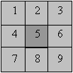
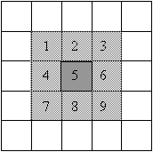
| kernel | Correlation: overlay and multiply |
Convolution: overlay, flip H&V and multiply |
 |
 |
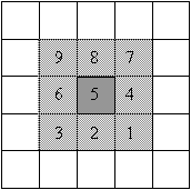 |
The only difference between these two equations is that there is a negative sign in front of the incremental indices for the kernel in the convolution equation. The negative signs alter the operation by rotating the kernel 180o prior to the pixel-by-pixel multiplication. Because all of the kernels we have used are symmetric about both axes, both operations produce the same result. The name 'image correlation' implies that there is some type of comparison going on between the image and the kernel. When identical shapes are overlaid there is a large positive correlation.
 |
|
In statistics there is a similar correlation computation that is used to determine whether 2 sets of data are related to one another, the result being the Correlation Coefficient. For 2 sets of data, data X and data Y, the correlation coefficient is computed via:
 |
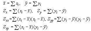 |
Statistical Correlation Coefficient Corr = 
|
This comparison can be done likewise for images. Using the statistical correlation calculation, we can use our kernel to select objects in the image that more closely match the kernel's shape, size and pixel intensity features. We refer to this selection kernel as the template image, so as not to confuse it with kernels used for noise filtering, and the process of using a template to select out objects in the image is called template matching.
Note that the correlation coefficient depends upon Sx and Sy, the average-corrected data, rather than on the data directly. On the imaging side, Sx and Sy are effectively the background-corrected pixel intensities in the kernel and in the image pixels under the kernel. By allowing for some pixels to take on negative values, the correlation value becomes much more sensitive to the kernel shape.
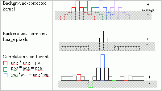
In addition, background intensity correction overcomes light intensity changes that often occur across the microscope slide and cause the image correlation values to likewise vary across the image even when the cells are similar.
|

|
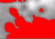
| Thresholded image after convolution with a disk kernel. | Elevated baseline and amplitude give elevated image correlation value. |
The denominator of the statistical correlation coefficient normalizes the result for changes in contrast amplification. Thus, if because of microscope setup, a portion of the image exhibited greater contrast such that cells in that region appeared with larger amplitude, those cells would also have a larger image correlation value. The denominator arises from the self-correlation of each image, equivalent to the standard deviation value, and thereby corrects for amplitude variations across different slides and/or across an individual slide. The statistical correlation value therefore matches image features by general size and shape. The Create-A-Template gizmo in ImageJ [ImageJ>Plugins>Create_A_Template] has an added button to allow you to compute the statistical correlation coefficient for each pixel in the image. You will have a chance to compare the results using this method with the standard image correlation results later in today's laboratory session.
As you will see, the statistical correlation operation performs very well in almost all cases. The following diagram demonstrates one possible scenario where the statistical correlation will give a false positive match. A template with a Gaussian-shaped pixel intensity distribution will generate a very high correlation coefficient for a region of the image containing a similarly-sized Gaussian feature. However, a 'hat' function of the same width as the Gaussian template will generate an even higher-valued correlation coefficient. In fact, any image feature having the same width as the Gaussian will give a favorable correlation.
 |

|
We may sometimes require a second source of information to further discriminate between
various objects in the image. For this we can turn to the gradient image. As a general rule,
the gradient operator acting on any dataset produces a resulting dataset that is different than
(orthogonal to) the original dataset. You have probably seen this previously in linear algebra
(i.e. quantum mechanics theory) and in studying Fourier theory – recall that the derivative of the
sine function is the cosine function and that the sine and cosine functions are orthogonal as far as
the inner product for the Fourier transform is concerned. To extract out the relevant features in
the gradient image we use a gradient template that is generated by taking the gradient
of the original template image.
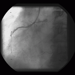
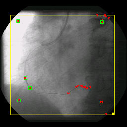
The combination of matching the image to a given template and matching the gradient of the image to a gradient of that template will prove to be very powerful for finding predefined objects in an image. The task remains though to create the best template for the job at hand. One of my prior research projects used template matching to find and track radio-opaque beads in X-ray fluoroscopy image. These beads are fixed to the tip of a balloon angioplasty catheter and the X-ray film catches the catheter as it is positioned and the balloon inflated in a coronary vessel of a cardiac patient. Or goal was to reconstruct the 3D anatomy and trajectory of the coronary vessel sitting on the heart surface and model its movement as a function of the cardiac cycle. [With this information we hope to be able to perform gated radiation therapy of the coronary vessels to prevent restenosis following balloon angioplasty. Without such treatment, 30% of all balloon angioplasty patients will present with critical restenosis within 3 months of treatment. However, with the application of relatively small doses of radiation the incidence of restenosis drops to < 10%.] An advantage of looking for beads under X-ray, as compared to cells under light microscopy, is that the pixel intensity profile of a 2 mm-diameter metallic bead can be easily modeled analytically. In fact, a Gaussian intensity profile works very well for finding these beads even in parts of the image where the CNR is relatively poor.
 |
|
The cells in your microscopy images are relatively circular and their sizes do not vary dramatically. In addition, there are not very many extraneous objects in the image that might confuse the template-matching algorithm, so a disk template may work satisfactorily for your present needs. However, it may also be of interest to you to be able to discern between cells of different shapes and textures, so perhaps a generic disk size is not sufficiently discriminating. There are perhaps several different solution strategies that will be successful for your ultimate task of counting and separating the cell types in your microscopy images. One you might find particularly clever both for its effectiveness and its simplicity…is ...
Since the template is an image itself, we are free to use any image pixel matrix
as the template. If we are fairly certain that all the objects in the image are
similar, then we can use the image of a representative object as the template.
Note: as you may have already discovered, there is a thresholding gizmo in ImageJ under [ImageJ>Image>Adjust>Threshold]. A thresholded image can be operated on by the built-in particle analyzer function [ImageJ>Analyze>Analyze Particles] to automatically count the number of thresholded objects in the image. I recommend setting the particle analyzer to Show> Outlines, and Display Results. Also, I have altered the disk kernel code to produce an inverted kernel image, compared to what was produced earlier.
- Try the Create_A_Template plugin on the demos3/testImage_small.jpg for a disk template with the radius set to match the size of the middle column of disks = 19 pixels. How do the statistical correlation values compare for the disks of differing intensity in that column? How do the correlation values change with disk size in the right column of the image?
- Try the Create_A_Template plugin for a disk template with the radius set to
match the size of a representative cell in the image – a trick for making the correlation
computation go faster for these trials is to reduce the size of the original image using
[ImageJ>Image>Scale]. The disk template radius will have to be
halved as well. Since the correlation operation takes ~ n2 operations, reducing the radius
by half will reduce the computation time by >Ľ.
- Can a single threshold setting be now used to pick out all the cells in the image? What is the rate of false positives (blobs that are not cells but that the template matching gives a high correlation coefficient to) and false negatives (missed cells)?
- The Create_A_Template plugin also has a button that lets you crop a
template image from the main image and use that for template matching. To use this, first
- Open the image and then open the Create_A_Template gizmo [ImageJ>Plugins]
- draw a box around the image object using the [ImageJ>taskbar>Box icon]
- click on the Crop Template from Image button and the template window should appear.
- now click the Perform Stats-Correlation button
- you may want to save that template image for future use. The Load Template from File button allows one to open any stored image file and use that as the template. [ImageJ>File>Save As]
- Do template matching to the gradient image
starting with the original image… - first prepare a gradient image for the disk template. -- create an appropriately-sized disk template using Create-A-Template -- compute the Gradient of this template using [ImageJ>Process>Gradient Analysis] and the default parameters (1 pixel step back and front in x and y directions and use magnitude) . -- save this gradient image as tiff using [ImageJ>File>Save As]
- back to the original image: first convolve it with a Gaussian filter to reduce the noise using the Create-A-Filter gizmo and a Gaussian kernel with a 7-pixel radius (=Gaussian standard deviation of +/- 1 pixel == the default setting), and hit the Perform Filtering via Convolution button. Hit the Done button to remove the filtering gizmo window since it is no longer needed. You can also remove the original image window and the Gaussian kernel window since these also are no longer needed.
- now perform a Gradient operation on the filtered cell image [ImageJ>Process>Gradient Analysis] using the default parameters.
- invoke the Create-A-Template gizmo [ ImageJ>Process>Create A Template] on the gradient image
- load the disk gradient image from the saved file using the Load Template from File button and perform a statistical correlation. You might want to save this image for comparison with the gradient template correlation you will generate next.
- Perform a correlation using a cropped template from the gradient cell image. You can use the same Create-A-Template gizmo that is currently active. Draw a box around a representative cell and make a template out of it using the Crop Template from Image button, then Perform Stats-Correlation.

