Optional Bonus Topic: Filtering in the Frequency Domain
-
Recap of Session I
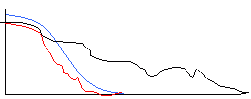
We learned last time of two important steps in the process of counting cells in the image. The first is to recognize when there is something of interest in the image by looking for regions of image contrast and object edges. The second step is to then identify these objects as being a cell versus artifact or debris based upon the object's relative size, shape, relative intensity and texture. We learned that a good way to have the computer highlight edges is through the gradient operator. We also touched on the concept of the contrast to noise ratio, CNR, which is a way to quantify our ability to detect edges in the presence of noise and artifact. {show UR lib image, take profile} [ImageJ > taskbar > Line Mode and draw across image] [ImageJ >Analyze >Plot Profile]. {Add noise and retake profile} [ImageJ >Process>Noise>Add Noise].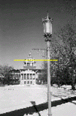
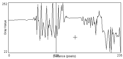
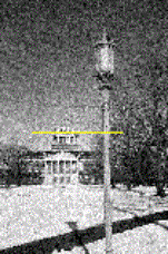
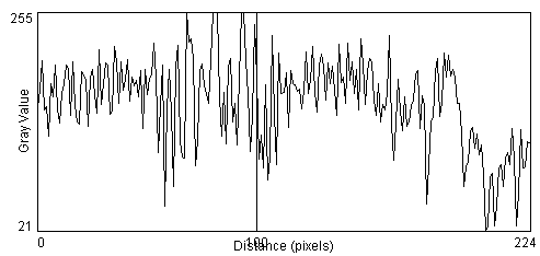
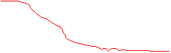
When we attempt to take the gradient of the image, the added noise dramatically degrades the results [ImageJ >Process>Gradient Analysis]. The standard gradient operation is very sensitive to noise because random fluctuations in image intensity from one pixel to the next look like sharp edges. {compare profiles across the lamp-post and its shadow in the gradient image with and without noise}.
- Image Noise
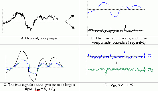
Today's session will consider ways to correct for noise in the image, or, in general, any signal. A generic definition of noise is any unwanted random signal. As a general rule, every time that a signal is processed in any way, noise is introduced. For most applications, the most important feature of noise is that it causes fluctuation in intensity from one pixel to the next and in the same pixel from one acquisition to the next. This is equivalent to saying that the noise is uncorrelated in both space and time. The first step in improving the contrast to noise ratio is to design the experiment so as to extract the cleanest possible signal. This you have already addressed in your cell studies by finding the lighting and contrast settings that give your microscopy images the clearest depiction of the cells. The second most popular thing to do to is to perform signal averaging. Consider the observed signal, S, to be comprised of the true signal, T, and a noise component, N: S = T + N
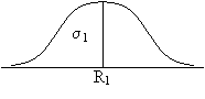
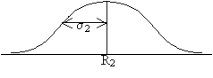
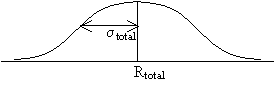
When the two true signals are added together, the total true signal is the sum of the individual signals. When the two noise components are added, however, the total resultant noise variance increases as sqrt(2). This result follows the laws of statistics when you are compounding measurements with expected errors given by a Gaussian distribution with variances &sigma1 and &sigma2.
Ttotal = T1 + T2 while &sigmatotal = sqrt(&sigma12 + &sigma22).
+ 
= 
Thus, when two noisy signals are added, the signal to noise ratio is expected to increase by: 2 / sqrt(2) = sqrt(2). If a signal is averaged n times the SNR increases by sqrt(n).Say you have a sound wave from coming from an audio CD-player that is being recorded onto a cassette tape. Suppose further that some noise (with variance s) is superposed onto the 'true' sound wave and is recorded as well. To reduce the noise, one could employ signal averaging by playing the CD a second time, recording that as well, and then taking the average of the two recordings. Since the underlying, 'true' signal should be identical each time, when the signals are added, the true signal components will sum to give a signal that is twice as large. However, because the noise component changes randomly each time, the added noise signals sum to some random, noisy signal whose amplitude is not as large as twice the individual signals. Thus, the overall signal-to-noise ratio goes up (by a factor of sqrt(2)).
- When presented with a single image, it is not possible to perform averaging over time. However we can perform spatial averaging, if we can assume that the intensity at a given pixel is somewhat related to that of its nearest neighbors. This will work if the true signal in neighboring pixels are at least somewhat correlated and the noise remains uncorrelated. In image processing, a simple way to achieve pixel averaging is to decrease the resolution of the image. In ImageJ we can do this by reducing the image size using the Scale function [ImageJ >Image>Scale] and then re-zooming to the original screen size. Using a scale factor of 0.5 reduces both the width and height of the image by ˝, there reducing the picture size Ľ. The effect is to average 4 pixels in the original image for every pixel in the resultant image. The SNR is therefore expected to increase by a factor of sqrt(4)=2. The same result could have been achieved earlier if you had simply reduced the resolution of the camera during acquisition.
- In today's lab session, you will have a chance to study a variety of signal averaging strategies, leading to some very powerful tools for image pre-processing that we will need to perform the subsequent cell recognition steps.
- When presented with a single image, it is not possible to perform averaging over time. However we can perform spatial averaging, if we can assume that the intensity at a given pixel is somewhat related to that of its nearest neighbors. This will work if the true signal in neighboring pixels are at least somewhat correlated and the noise remains uncorrelated. In image processing, a simple way to achieve pixel averaging is to decrease the resolution of the image. In ImageJ we can do this by reducing the image size using the Scale function [ImageJ >Image>Scale] and then re-zooming to the original screen size. Using a scale factor of 0.5 reduces both the width and height of the image by ˝, there reducing the picture size Ľ. The effect is to average 4 pixels in the original image for every pixel in the resultant image. The SNR is therefore expected to increase by a factor of sqrt(4)=2. The same result could have been achieved earlier if you had simply reduced the resolution of the camera during acquisition.
-
Lab session #2
-
Signal averaging by decreasing spatial resolution
Repeat the scaling by 0.5 and re-zooming procedure on one of your cell images. [ImageJ>File>Open] [ImageJ>Image>Scale], using a value of 0.5 to start Zoom using [ImageJ>taskbar>Magnifying Glass widget] Starting with the original cell image, repeat the scaling but this time using scale values of 0.25 and/or 0.125, and zooming accordingly. Take profiles for each [ImageJ>taskbar>Line Drawing widget] [ImageJ>Analyze>Plot Profile]. You could save the data of the profile using the save button on the Profile Plot screen, but we do not need this data at the moment. You can also save an image of the Profile Plot by first bringing the Profile Plot screen to the front by clicking on it, then save it as jpg via [ImageJ>File>Save As]. Save a couple of the more representative profiles for inclusion in your lab book. You should notice that the profiles become much smoother (i.e. the noise is reduced) as the resolution is decreased, but your ability to discern objects in the image gets much worse – note the degradation of the time stamp in the upper-left corner. It would be nice to perform signal averaging without as large a loss of effective resolution. - Sliding window method
An improvement over the method of increasing the pixel size in the image comes with the use of a sliding window averaging technique. Rather then average 4 pixels to one larger pixel, and then shifting your attention to the next 4 pixels, the sliding window method uses the same pixel sizes as the original image, but for each pixel you take the average of that pixel and it's nearest neighbors. The following diagrams should define the differences in the methods, for the 1D case and a 3-pixel-wide window: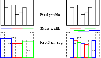
In ImageJ, iteration over the entire 2D image is performed via: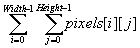
For a slider width of 3 pixels in the width and height directions (note: the width should be an odd number to put the target pixel directly in the center), the equation for the resolution reduction method can be written in Java as:
float[][] pixels = new float[Width][Height];
float[][] avg = new float[Width/3][Height/3];
//  get the pixels matrix values from the current image on display
pixels = MathII.getCurrentImageMatrix();
for (i=1; i < Width-1; i = i+1 )  {  // width of image
   for (j=1; j < Height-1; j = j+1) {    // height of image
       avg[i][j] = (float)0.0;  // the resultant, average
       for (m=-1; m < =1; m = m+1)  {  // width of averaging 'kernel'
          for (n=-1; n < =1; n = n+1)   {  // height of averaging kernel
	   avg[i][j] = avg[i][j] + pixels[i+m][j+n];
          }  // end of n loop
       }  // end of m loop
   avg[i][j] = avg[i][j]/(float)9.0;
   }  // end j loop
} // end I loop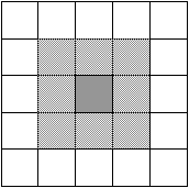
test image Note that we divide by 9 because there are 9 pixels being averaged.
In ImageJ, there is (now) a gizmo to perform the sliding window method, allowing the user to define the kernel size and shape and then apply this filter to the image: [ImageJ>Plugins>Create A Filter].
- open one of the cell images. Note: some of the PC's in the lab are rather slow. To help speed up things for these tests, you can work on a smaller representation of one of the cell images using [ImageJ>Image>Scale]. I recommend scaling it by 0.5 in each direction, creating an image that is only Ľ as large. Because the filtering operation requires roughly (npixels)2 mathematical calculations, a smaller image should take only 1/16th as long to work on. I also recommend that you then save the shrunken image with a clever name (e.g. cells_small.jpg) so that you won't have to go the scaling procedure every time you need to start with a new image.
- set the Hat Width and Hat Height to 3 (use 7 if working on a full-size image) 7 and click the Create Hat Kernel button to create the filter on the computer (the image of the filter has been zoomed in automatically to enable us to see it better – you can unzoom it a couple times (read the zoom factor in the title bar of the kernel window) if you want to see its true size compared to the original image. Now hit the Perform Filtering via Sliding Window button. Note how the smaller bubbles in the background disappear. As a general rule, objects that are smaller than the filter are lost.
- Set the filter width to 3 (7 for full-size image) and the filter height to 0. Note how the image looks blurred in the X-direction (=width), as if the microscope was shifted from right to left during the cell image acquisition. This filter similarly mimics the image blur resulting from a uniform horizontal motion of a camera. This is also the same filter I used to create the blurred version of the photograph of the UofR undergrad library shown earlier (you can do it yourself on the library image if you have time). Correspondingly, correction of motion-blurred images is achieved using the inverse of this filter (done in the frequency domain though).
- We should now step back and re-consider the operation we just performed in the image. One minor problem is that we give equal weight to each of the pixels surrounding and including the pixel of interest. One would imagine that the pixel intensity at the pixel of interest is slightly more representative of the true intensity there than the pixel intensity of the surrounding pixels, especially the ones at the corners whose centers are farthest away from the center of the pixel of interest.
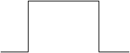
"Hat" Function Gaussian Function -
Gaussian filtering
A more ideal signal averaging function might be one that gives individual weights to the neighboring pixels, perhaps depending on the distance of the center of each pixel from the center of the pixel of interest. For this purpose, a Gaussian weighting function is commonly used.
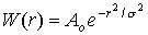
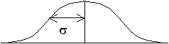
Equation of Gaussian 2D Gaussian Profile 'r' is the distance from the center of the pixel of interest to the current pixel, Ao is a normalization factor, and &sigma2 is the standard deviation (~width) of the Gaussian profile. The digitized version of a typical Gaussian weighting function is shown above for the case of the Gaussian being twice as large in the height direction than in the width direction. The matrix form of the weighting function is called a kernel. The Gaussian kernel is scaled by Ao such that the sum of all the contributions is 1.0. In the previous example, the sliding window defined a 'Hat' kernel with Ao equal to 1/9. Note that the Gaussian kernel is sampled out to a sufficient distance such that the weights at the edge pixels are sufficiently close to zero. In the kernel shown above, the distance in the width and height directions is equal to 3* &sigmaw and 3* &sigmah, respectively. Ao is computed simply as 1/(the sum of all the kernel elements). Going back to the equation/code that was derived earlier, for arbitrary kernel width (or height) = z, which for a Gaussian kernel = 2*(3*&sigma) + 1:
// first zero the avg matrix to take care of the edges
for (i=0; i < Width; i += 1 )
   for (j=0; j < Height; j += 1)
      avg[i][j] = (float)0.0;

for (i=(z-1)/2; i < Width-(z-1)/2; i += 1 )  // width of image
   for (j=(z-1)/2; j < Height-(z-1)/2; j += 1)  {   // height of image
        kw = 1; 				 // the width index to the kernel
        for (m=-(z-1)/2; m < =(z-1)/2; m += 1)  {  // width of kernel
             kh = 1; 			 // the height index to the kernel
             for (n=-(z-1)/2; n<=(z-1)/2; n += 1)  {  // height of kernel
	      avg[i][j] += kernel[z-kw][z-kh]*pixels[i+m][j+n];
	      kh++;
              } // end n loop
              kw ++;
         } // end m loop
    }  // end j loop
Note that I took pains to show a minor change to the equation that you derived earlier, namely that I now increment the kernel matrix from high to low index ([z-ki][z-kj]), i.e. from right-to-left and bottom-to-top across the matrix elements, rather than the usual left-to-right and top-to-bottom. Because the Gaussian kernel is symmetric, this will not affect the result, however this puts this equation into a more common notation, that of the image Convolution operation. Image convolution is a very powerful and oft-used tool in image processing. Our strategy for recognizing objects in the cell images now begins by convolving the image with a Gaussian kernel prior to performing a gradient operation. The noise reduction step is now part of the image pre-processing steps. The Create A Filter gizmo in ImageJ also allows you to define a 2D Gaussian kernel and convolve that with the original cell image. The user sets the width and height of the Gaussian kernel in pixels, and s is computed internally according to the equation above: z = 2*(3*&sigma) + 1, or &sigma = (z-1)/6 . Note, elliptically shaped Gaussians (as shown in the figure above) are perfectly legal, but I limited the gimzo to produce axisymmetric Gaussians for simplicity.
-
Back to the lab…
-
open one of the cell images and compute the gradient using the default parameters (1
pixel step in each direction and use the magnitude)
[ ImageJ>Plugins>Gradient Analysis ].
- go back to the original cell image and perform the Gaussian convolution using
the new gizmo: [ImageJ>Plugins>Create_A_Filter] using a
kernel width and height of 7 pixels (this corresponds to a Gaussian filter with s = 1 pixel).
Note that the image looks blurry to your eye. Now perform the same gradient computation
as before, but to this filtered image. Even though the edges might appear less distinctive
to your eye, the gradient operator was able to find them better than before the Gaussian
filter was applied. In addition, the background noise in the gradient image is
significantly reduced!
- starting again with the original cell image, apply the Gaussian filter using a
kernel size
of 15 pixels in each direction, and compute the image gradient as before. Compare this to the
2 previous gradient images. What happened to the medium-sized bubbles in the background?
The cells in the image are approximately 40 pixels wide. What would happen if we used a
40 pixel wide filter?
One should also consider the relationship between the filter size and the gradient kernel size, and finding an optimal matching of the two, but we will not delve into that at this time.
- Finally, there is another kernel shape available in the Create-A-Filter gizmo -- you
can arbitrarily specify a disk-shaped kernel to run the convolution/filtering operation on the
main image. First try this for a radius of 4 pixels, to match the earlier runs. Next try this:
- Open one of the cell images in the demo directory
- Measure the width (in pixels) of one of the cells. You can do this using the line drawing tool [ImageJ>taskbar>Line Drawing widget]. When you draw a line, the ImageJ window shows the current cursor position and the current length of the line.
- set the radius for the disk kernel to match the well width (width/2)
- create that kernel by clicking the Create Kernel button
- filter the image using this kernel by clicking the Compute Convolution button
-
open one of the cell images and compute the gradient using the default parameters (1
pixel step in each direction and use the magnitude)
[ ImageJ>Plugins>Gradient Analysis ].
-
Signal averaging by decreasing spatial resolution
-
Optional Bonus Topic: Filtering in the frequency domain
So far we have looked at the filtering process by considering filtering functions (kernels) of varying shapes and sizes, but there is a way to perform the same filtering analysis considering only the frequency components of the images and the filters. Not surprisingly, these will eventually lead us to the same conclusions, but it is none-the-less interesting to look at the problem from a different viewpoint. I will not attempt to be very rigorous or very thorough here, but by the end of this section you should be able to understand the principle concepts. The classic filtering problem occurs in audio signal processing where the signals of interest (sometimes known as music) are often corrupted by tape hiss, acoustic noise from the electronics in the amplifier, etc. The classic noise source is the electrical system of modern buildings that have a wall AC current supply that comes in at 60Hz. This noise source becomes especially problematic in rooms with fluorescent lights and for radio station in the AM dial (where all the best stations reside!). In this case, since we know the frequency of the noise source we can design filters to preferentially remove all of the signal coming in at 60hz. Most often we do not know exactly the frequency of the noise, but the noise usually is a bigger problem at higher frequencies. Tape hiss is a good example. The most effective audio filters are those that manage to filter out the signal at the higher frequencies while preserving the signal in the middle frequencies where the human voice and most instruments are found. In 2D images, noise usually presents as speckles in the background of the image. These speckles occur because the noise in one pixel is generally uncorrelated with the noise in neighboring pixels.
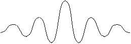
- Frequency content and slopes in the image
From some previous class on Fourier theory you may recall that objects with very sharp edges (large slopes) require higher frequencies to reconstruct them. For the Gaussian bump illustrated below, imagine trying to reconstruct that using sine and cosine functions. A very long (low frequency) sine wave could do a pretty good job for a broad bump, but a higher frequency sine wave would be required to fit a narrow bump.
Gaussian Bump 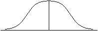

Sine waves 
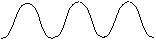
low freqeuncy high freqeuncy When you look at the frequency content in an image, images with objects that have sharp, narrow edges have lots of high-frequency content, while images that have only objects with broad edges have very little high-frequency content. Noise speckle is a very high-frequency feature because noise represents large image intensity differences over a very short distance (usually over only a single pixel). In general, when acquiring an image one tries to set the resolution such that the objects of interest are many pixels wide. This results in the frequency content of the objects of interest being lower in frequency than the background noise. All of the filtering methods used earlier worked primarily by removing the high-frequency components in the image. Recall from the first lecture the diagram showing the radiation dose profile of the tumor and how I modeled the effect of tumor motion on the radiation dose observed by the tumor during treatment. The model I used was very similar to the sliding Hat filter. The effect of tumor motion was to erode the radiation dose profile by reducing the sharpness of the dose up-slope at the tumor edges and reducing the total magnitude. I modeled this by convolving the original dose image by the Hat filter. Reduction in the slope of the radiation dose is a direct result of filtering out the high-frequency components, leaving only the low frequency components that cannot reconstruct as sharp an edge. In the image filtering operations you performed earlier, you achieved the same results. Applying a filter always blurred out the cell edges. The positive effect was a reduction in the magnitude of the background noise.
- Gaussian filters and their frequency content
The classic noise filter is a simple low-pass filter that removes all of the signal at frequencies higher than a prescribed cut-off.
Frequency content (Spectra) of original image 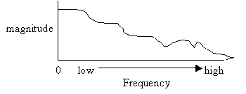
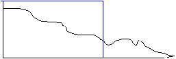
cut-off freq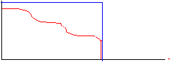
The disadvantage of this simple approach is that the frequency cut-off is very abrupt while the frequency content of the true signal falls off slowly. The abrupt frequency cut-off can also lead to many types of image artifact (Gibb's Ringing is a common artifact in MRI). A more desirable frequency filter would be one that falls to zero more gradually.
more ideal filter 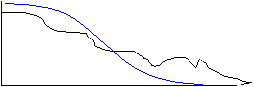
Note that in these diagrams the frequency curve in the resultant diagram was computed by multiplying the frequency curve of the original image by the frequency profile of the filter. In the first case the multiplication was by a 'Hat' function with amplitude of 1 inside the 'Hat', giving a resultant frequency curve that was identical to the original for frequencies lower than the cut-off, and 0 for frequencies above the cut-off. In the second case, the frequency curve in the resultant diagram was computed by scaling down the original curve so that it fit within the 'envelope' of the filter curve. There are many types of filters that falloff gradually, but we will consider here only the Gaussian filter. A unique feature of a Gaussian profile is that for a Gaussian curve in imaging space with a width (variance) of &sigma, the Fourier transform is a Gaussian curve in the frequency domain with variance ~ 1/&sigma. Thus, a narrow Gaussian kernel in the spatial domain transforms to a broad Gaussian curve in the frequency domain, and visa-vera.
[The real beauty of looking at things in the frequency domain is that convolution in the image space (spatial domain) is equivalent to multiplication in the frequency domain. Thus, the lengthy calculation you derived for with convolving the cell image by a Gaussian kernel could have been replaced by a simple, straightforward and fast multiplication in the frequency domain.]
Broad freq filter Narrow freq filter 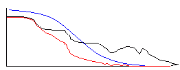
A broad Gaussian kernel in the spatial domain translates to a narrow filter in the frequency domain. A filter with a narrow frequency width effectively removes a lot of the high frequency content, which would cause a large reduction in the slope at the cell edges, and this is what you observed when you convolved the cell images with a Gaussian filter with a wide kernel. Likewise, a small kernel convolved with the image preserves much of the high-frequency content, preserving the cell edges, but does not remove much of the background noise.
Another advantage of the Gaussian filter over the Hat filter is that although the Hat function looks nice in the spatial domain, it transforms to a wacky sinc (= sin(x)/x) function in the frequency domain. This gives incomplete reduction of high frequency noise and alters the features of the image in hard-to-understand ways.

Hat function in spatial domain Fourier transform Sinc function in frequency domain ImageJ has a fast Fourier transform (FFT) feature and the inverse FFT. You can use this to take the fourier transform of a 2D disk function (analogous to a hat function in 1D). That image is called smallDiskImage.gif. Perform an FFT on that [ImageJ>Process>FFT / invFFT]. Display the real part of the FFT with the Volume Center box checked. The pixel at the exact center of the FFT image has a very high value – this is the zero-frequency, or DC, component of the image == the average of all the pixels in the image. Do a plot the pixel intensities along a line that just misses this central peak [ImageJ>taskbar>Line Drawing widget] [ImageJ>Analyze>Plot Profile]. You should see a sinc-like function. There is a second disk image: bigDiskImage.gif you should also do an FFT on.
It would be interesting to be able to compute and display the FFT of the cell images and to be able to crop out just the center of the fourier space, or all but the center, and take the invFFT of that.
- Frequency content and slopes in the image