{Note: many of the demos used herein rely on the NIH ImageJ program (a java version of NIH-Image for use on virtuallyany computer system). This program and the source code can be downloaded for free from: the NIH ImageJ web site.}

1. Introduction and background
   digital image and matrix data
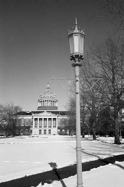
   In review, a digitized image is simply a bunch of numbers assigned to an array (a 2D array in this case) and displayed so that the intensity of each array element corresponds to some value of interest at that position. In the computer, an image is usually stored as a matrix, where each array element then is an element in the matrix, and is stored in a logical fashion such that the top left corner of the image is in matrix element [width=0][height=0] and the bottom right corner of the image is then [ImageWidth-1][ImageHeight-1]. The coordinate x is usually used to refer to the width (row) index, and y the height (column) index. In a two-dimensional image, each matrix element is called a pixel (short for picture-element). The process of converting an analog image to a digitized one is often called pixilating the image. This is also known as digitizing or sampling. In three dimensional image sets, each array element is called a voxel (short for volume-element). Most people are familiar with images where the pixel intensity corresponds to the amount of light emanating from the imaged object, such as this photo of our beloved campus library {see UR lib image}. The individual pixels can be discerned better when we zoom in on the picture.
   

   UofR Campus Library	Axial CT image of a lung	Sagittal MRI image of the same lung

   In many medical applications, pixel intensity corresponds to other attributes of the subject. In CT (computed tomography), image pixel intensity corresponds to the X-ray opacity of the tissue {see lung CT image image}. Dense tissues, such as bone, block much of the x-ray beam going through the body and to the receiver. For CT imaging, a back-projection algorithm is used to compute the radio-density of the tissue at every pixel in the image to create the axial image slice seen here. This CT image set was acquired in a lung cancer patient and one of 5 tumors in this patient's lung region can be seen at slice #39. In the CT images, we can discern the bone, the skin, the fatty layer under the skin, muscle tissue and lung tissue. In these images we can also discern the surface fiducial markers used to help register the images with other images sets, such as the corresponding magnetic resonance imaging (MRI) studies. In MRI, pixel intensity corresponds to the amount of water in the tissue {see lung MR image}.

   However, pixels intensities do not necessarily have to correspond to an imaging parameter. Any matrix can be displayed in image form. For this same cancer patient, a radiation treatment plan was made to expose the tumors to high doses of radiation. The amount of dose going to each tumor and the surrounding lung tissue can be computed, say at every millimeter in each direction throughout the patient's body, and the dose values can then be stored in a matrix and displayed as an image. The advantage of thinking of the dose distribution as an image is that there are many powerful computational tools that have been developed to extract information from digital images that can also now be applied to the dose field. {see dose volume}. For example, we can now use this method to predict the effect of breathing motion on the dose seen by the tumor. We do this by modeling the effect of tumor motion as we would model the blurring that is observed in a photographic image when the camera is moved during the exposure. {see UR lib image} {see blurred UR lib image}

   UofR Campus Library	library image with motion blurring	image after blurring correction (top half)

   We can model this effect using image convolution theory, which we'll learn more about later. But for now, it suffices to say that this method allows us not only to blur an image to simulate camera motion, but also to partially un-blur an already-blurred image to correct for a known image distortion. {see motion-corrected UR lib image} For the radiation dose field observed by a tumor that is moving while the radiation beam is turned on we get the results shown in the following figure showing the dose intensity profile across the center of the tumor after we model the tumor as moving +/- 4mm in the radiation field, {see dose distribution image and dose profile graph}. Our hope is that by better understanding the blurring of the dose field seen by the moving tumor, we can modify the way we prescribe and deliver the radiation so as to ensure that the entire tumor is being exposed to a lethal dose, while also ensuring that the surrounding healthy lung tissue receives as little dose as possible. Also, just as treating physical data as an image gives us new ways to perform data analysis using image processing techniques that have been developed over the years, treating an image as a matrix of numbers gives us powerful tools from vector algebra that can be applied to image analysis.

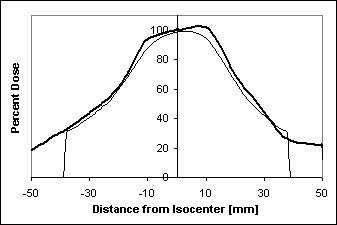
   Radiation dose distribution around tumor	Dose profile across tumor center with and without [bold line] tumor motion

   Image processing books that I have used recently and that are available at the CSE library:
   

   Press, W., et al., Numerical Recipes in C, The Art of Scientific Computing. 2nd ed. 1988, Cambridge, England: Cambridge University Press.
   
   Andrews, H.C. and B.R. Hunt, Digital image restoration. 1977, Englewood Cliffs, N.J.: Prentice-Hall. 238
   
   Bates, R.H.T., Image restoration and reconstruction. 1986, New York: Oxford University Press. 288.

   Our task in the next 2 weeks is to take the microscopy images you will later acquire and develop an algorithm to automatically detect and count the number and types of cells in your samples. For some of these images, detecting and counting the cells may not present an overly difficult task given the small number of cells and the fact that they are usually well-defined and separated from each other, but as we are developing our methods we should keep in mind the ultimate task of dealing with images containing perhaps hundreds of overlapping cells of various sizes and shapes. Also, your algorithm should be able to handle images that may contain much more noise or debris in your microscopy field.

   ---

2. Human Perception
   Your eye's (and brain's) ability to perform image feature detection

   

   When you look at this image and are asked to locate all the various cells, you immediately point to each individual cell, and you are almost always correct in your choice. But how does your brain do that? In our field, we are often asked to design tools and devices that are intended to mimic, or sometimes even to improve on, the function of the human body. This is one of those instances, and you'll find it helpful to consider some of the types of processes that your brain uses to perform object recognition. For instance, we should first ask ourselves: what features of the objects in the microscopy image make you identify them as being something that deserves your attention?

   We can list several of these:

   • Relative darkness or lightness (contrast)
   • Sharp Edges (gradients)

   Second, what features of the objects make you identify them as an object of a particular class?
   We should list several of these:

   • Relative size
   • Shape
   • Relative darkness or lightness
   • Texture

   A major identifying attribute is pixel intensity constrast relative to the surroundings. It should not surprise you that your eyes and brain have the ability to perform background subtraction and edge detection capabilities very early on in the processing of visual information. First, before the visual signals even leave the retina, the visual cues coming from each rod cell are modified to accentuate image contrast. As you can read in the excerpts from the Textbook of Medical Physiology by Guyton, each rod cell has a central excitatory zone surrounded by an inhibitory zone. The effect of this bi-phasic response is to improve our ability to detect differences in image intensity from one rod cell to the next, and this also acts to reduce our attention to areas where the image intensity is constant across a large region. In other words, the retina performs the initial image processing steps of background subtraction and edge enhancement. The deeper parts of the brain then add to this enhancement and look for additional features such as object shape and motion across the visual field.

   Guyton's physiology textbook:
   

   Guyton, A.C. and J.E. Hall, Textbook of Medical Physiology. 10th ed. 2001, Philadelphia: Saunders. Chapter 51, p586-590

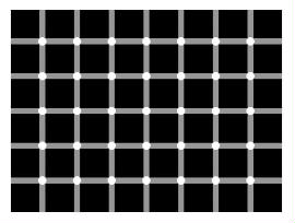
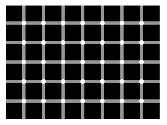
   The 'Dots' illusion: counts the dots :P Your eyes are performing background subtraction to create the illusion of dots between the squares.

   more illusions: http://www.exploratorium.edu/exhibits/f_exhibits.html (I highly recommend the 'death spiral' -- look at something else immediately after gazing at the spiral)

   ---

3. Edge Detection
   
   An edge in an image is an abrupt change in image intensity, presumably at the boundary between differing materials. We can characterize the edge by considering both the width of the edge, and the magnitude and sign of the intensity difference. In ImageJ we can use the Plot Profile function to plot the image intensity across the object of interest. [ImageJ > taskbar > Line Mode and draw across image] [ImageJ >Analyze >Plot Profile].

   An important and often overlooked parameter in image processing is the concept of the contrast-to-noise ratio. You are probably familiar with the concept of the Signal to Noise Ratio (SNR) which is the ability to find the signal in the presence of noise, but here we are not so much interested in whether the background light intensity is much higher than the noise, as we are interested in whether we can find the cell edges within the image, in the presence of noise [ImageJ >Process>Noise>Add Noise]. When more noise is added it becomes nearly impossible to discern object edges across the profile line, even though our eyes are still good enough to detect the pole in the image, using shape information gathered over larger regions of the image.

   So how do we quantify the edges in the image in a manner that can be performed by a computer? Since the edge is defined a sharp change in the image intensity over a relatively few number of pixels, a simple method is to compute the slope of the intensity profile at each pixel. There are several methods for computing a slope and we should investigate several of these to discern which is most appropriate for our current application. A commonly-used approach is to compute the magnitude of the slope at the pixel of interest, as determined from consideration of pixels on one or both sides of pixel of interest. This is called computing the Gradient of the image, is usually done in 2D, and the computation of the gradient of the image is called performing a Gradient Operation on the image. In lab we will investigate further the properties of the image gradient operator.

   ---

4. Lab session #1

   For the first lab session, you should first familiarize yourself with the ImageJ program. ImageJ is meant to be an easy-to-use image processing tool. It is based on the program NIH Image that was written for and became popular on Macintosh computers. ImageJ is written in Java language by the authors of NIH Image and who still reside at the NIH. Because ImageJ is written in java it can be compiled and run on virtually any computer system. It has an official web set at: http://rsb.info.nih.gov/ij/ where you can look up the latest examples, documentation, and plug-ins. It is designed to be modular, meaning that individual users are encouraged to write their our small programs (plug-ins), and these can be automatically compiled and incorporated into the ImageJ program without much additional effort on the users' part. ImageJ is very similar to Scion Image in many respects. One difference is that (apparently) Scion image can handle only Tiff, BMP and Dicom image formats, while ImageJ handles virtually any image format (Tiff, Gif, JPG, BMP, Dicom, etc). Scion's drawing tools are better than ImageJ though. A very nice feature of ImageJ is that it is entirely free and open source -- meaning that you have full access to all its source code. This is a great help when trying to modify their code or to write your own code from scratch since you have many working examples to look at.

   I recommend trying to repeat the analyses performed during the lecture session. Have a look at all the demo images and try some of the features demonstrated earlier: loading a single image, loading an image series, zooming in and out, drawing a line and plotting an intensity profile along that line, adding noise, setting the window and level, etc.

   The Window and Level gizmo
   The Window value assigns the spread in the gray-scale values represented in the display. The Level sets the middle of the range, i.e. the intensity value in the original image that will get the middle gray-level value (128) in the transformed image. To showcase this,

   1. open the tumor dose image [ImageJ >File>Open>tumorDoseImage.gif]
   2. convert the image to grayscale [ImageJ >Image>Lookup Tables>Grays]
   3. invoke the histogram function on this [ImageJ >Process>Gradient Analysis] This histogram window shows the range of radiation dose values present in the data: 0 to 158, and the gray scale intensity bar used to present the data as a gray-scale image. Note that the maximum dose value of 158 is set to a medium-light gray-level value, and correspondingly the image is rather dark.
   4. now invoke the Window/Level gizmo [ImageJ >Image>Window and Level] Invoking Window/Level automatically sets the Level to equal the middle of the dose range and sets the Window value such that the lowest dose value (0) to black, and the highest dose value (158) to white.
      
      A trick for using the Window and Level gizmo is to first set the Window value to its lowest setting. This will force the pixels to take on either white or black values, depending on the Level value. All pixel intensities in the original image that are below the Level value will be black, and all those above the Level value will be white. This is equivalent to setting a threshold value.
   5. set the Window value to 1 and the Level to some random value, say 37. Now invoke the Contour Plotting feature [ImageJ >Analyza>ContourPlotter]. This will draw isocontour lines on the image at the given levels when you hit the Make Contour Plot button. For contour Level #1, enter the value used for the Window/Level Level value (e.g. 37) and make the contour plot. The line between the white and black pixels should match the green isodose contour.
   6. Now go back and adjust the Window value and you should observe the grayscale values across the image changing, but the gray-level value at the green isodose contour remaining at mid-gray (128).
      
      Back to the trick: With the Window set to its lowest setting, adjust the Level so that you can readily discern the features of the image that you are interested in. Once you are happy with that setting, go back and adjust the Window value to achieve nice image. The Window-Level gizmo operates only on the image window that was on top when the Window-Level gizmo was originally invoked.

   Gradient Operator:
   A separate plug-in has been created to allow one to compute the gradient of an image using any of a number of user-defined parameter settings [ ImageJ >Process>Gradient Analysis ]. The plug-in allows you to compute the unidirectional gradient in either the X-direction or the Y-direction, or to compute a 2D gradient, with magnitude defined as the sqrt(G_x² + G_y²). For the unidirectional gradient calculation, you can set whether to use the slope of the intensity directly, or to use the magnitude (absolute value) of the slope. You are also able to set the width (in pixels) of the region over which the slope is computed.

   1. Start by computing the X-directional gradient. Set the Y-direction forward and backward steps to 0. The slope in the X-direction is computed by performing a linear regression analysis using the pixel intensities for those pixels located between xSteps to the right of the pixel of interest and xSteps to the left. You may want to use the Window and Level gizmo after performing many of the gradient operations since the largest image intensity of the gradient image will likely be much less than that for the original image. A Window and Level gizmo is created automatically for this window when the gradient gizmo is created.

   2. Set the "Display magnitude" off. The result is often called a watermark effect. Changing the ratio of the x and y steps changes the angle of the 'shadows' in the watermark. Perform the gradient operator with the "Display Magnitude" back on for the rest of the trials.

   3. Increase the width to the gradient zone by increasing the step sizes. By increasing the zone, you are tailoring your edge detection scheme to highlight mostly those features in the image with edges that rise over a similar distance. However, the price you pay is that edges that occur over much smaller distance than the zone width are smoothed over.

   4. How does the gradient operator affect your ability to determine the exact location of the edge of the cell? i.e. use the line Profile Plot feature on the gradient image and try to match the feature in the gradient profile that best matches the edge in the original image.

   5. Add noise to the original cell image via ImageJ >Process>Noise>Add Noise, now take the gradient. Next session we'll try some methods to overcome image noise without significantly degrading the results of the gradient operation.
      Try the gradient operator also on the test image (demos1/testImage.jpg).

5. Optional Bonus Topic: Snakes

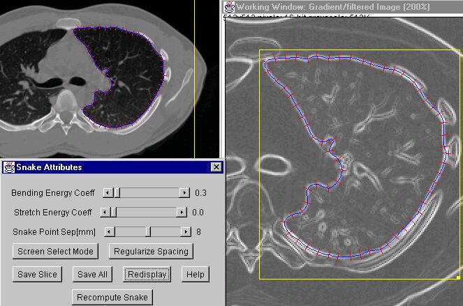
   Segmentation of image objects is a critical issue in many medical imaging applications, such as in delineating and mapping different structures in the brain (caudate nucleus vs thalamus vs tumorous mass). Around 1990 a novel technique came into being wherein a mathematical construct for a piecewise curve in space was combined with a mechanical model of the stretching and bending forces of a spring to construct a deformable contour model, also known as active contours, and known in the business simply as snakes. The basic idea of a snake is that one desires a contour line to be able to respond actively to the information provided in the underlying image, but also to have some built-in constraints to prevent the contour line from being led into doing wacky, non-physiologic things, like contorting into a pretzel shape when we all know that the surface of the heart is relatively elliptical by nature. The ultimate goal would be for the user to be able to draw an initial, simply shaped contour near the image object of interest, and then have the contour automatically resize and reshape to match the image object.

   First, the contour line is defined as a sequence of nodes connected by spring-like connections. The driving force behind the movement of the contour line to the image object is usually taken to be an attraction of each node toward the object boundaries, i.e. the magnitude of the gradient operator acting on the original image. Thus an energy term is associated with each node wherein a low energy state exists when a node is sitting on a bright spot in the gradient image -- the external energy term. The constraints to the contour shape are created by associating high energies whenever there is a sharp bend in the contour line and/or whenever two nodes become spaced either too far or too close from/to their neighbors - the internal energy term. The object for the snake then is to work toward the minimum energy state, that is, once in which the contour line lies on or very close to the image object at all nodes, yet retains a relatively smooth shape.

   A snake is a 2D active contour; in 3D, the active contour is often called a balloon. As the name implies, the user typically draws a spherical 'balloon' entirely inside the object of interest, then the 'balloon' is allowed to 'inflate' and fill up the interior of the image object in all directions, until the object edges are meet. Often one has to tweek the relative strength of the external versus internal energy terms to optimize the snake to meet a particular segmentation need. If there is no underlying image feature information, then the snake will take on a circular shape (minimizes both binding and stretching). If there is no internal energy term, then the contour line will often take on a very irregular shape; responding to any noise or gap in the image feature information. I created an interactive snake gizmo in ImageJ for the purpose of segmenting lung contours in the diagnostic CT/MRI images. The gizmo allows the user to adjust the relative internal and external energy coefficients, and other parameters of interest, on-the-fly while observing the result on the screen. The program is clever enough so that once one slice has been completed, that snake geometry is used as the starting point for the next image slice, and so on. The program I wrote has some problems at times, but beats doing it all by hand.

   

   Try the snake on the test image first (demos1/testImage.gif). To use the program, you must first open an image and draw a box-shaped (or oval-shaped) region of interest (ROI) around the object of interest, then invoke the procedure (ImageJ > Process > InterActivesnake). The incomplete disk at the top-left illustrates the utility of having internal energy terms to interpolate over gaps in the image data. The blob in the middle left-side is good test for convergence of the snake. Try the program also on one of the lung CT images (demos1/lungLesionCT/37.img) and try to segment one of the lungs.